Costumer segmentation

Customer segmentation is the process by which you divide your customers up based on common characteristics – such as demographics or behaviors, so you can market to those customers more effectively.

In this notebook I will try to develop a comprehensive example in order to cluster customers in different bins, this will include :

  • Data exploratory skills with Pandas, Numpy and Matplotlib
  • Data cleaning and a little bit of feature engineering though Pandas mostly
  • PCA implementation and how to correctly choose dimensional reduction based on cumulative variance
  • Clustering implementation with unsupervised ML algorithm using Kmeans and the Elbow method. 

Uncommon libraries used in this notebook :

from yellowbrick.cluster import KElbowVisualizer

I used this library that is very user friendly to find the right clustering with the K elbow method.


Data Cleaning

Here we are performing data cleaning tasks that are detailed bellow thanks to the experience accumulated cleaning multiple Dataframe this task was not really challenging so I will pass quickly on it.

def per_missing(df) : 
    # Create the serie with missing values : 
    missing_values = df.isnull().sum()
    non_missing_values = df.count()
    per_miss = missing_values/non_missing_values*100
    return per_miss

print(per_missing(df)[:10])

# 1 % of the income feature is missing, we can fill the values with most comon, mean, median or even with a machine learning algorithm. 
# Here are probably going to use the median and change if the results are bad. 
# Filling the NaN or Null values with the median 
df['Income'].fillna(value=df['Income'].median(), inplace = True)
print(per_missing(df)[:10])


Important part during your clustering process :

Detect and address the outliers of your DataFrame, those outliers will have an impact on your Standard Deviation, they will have an impact on your mean.

Therefore your segmentation will be overly impacted by few case taht are not really relavant here.

Feature engineering

Here nothing crazy, we are simply going to add some attributes and remap some variables, the point is :

  • To simplify some attributes who contains a level of complexity that is not going to help our model
  • Extract a feature based on other features to add useful information for our clustering
# Create the Age attribute : 
df['Age']= max(df['Dt_Customer'].dt.year) - df['Year_Birth']

# Create the Total_spent attribute : 
df['Total_spent']=df['MntWines']+df['MntFruits']+df['MntMeatProducts']+df['MntFishProducts']+df['MntSweetProducts']+df['MntGoldProds']

#Create the Eldership attribute :
last_date = max(df['Dt_Customer'].dt.date)
df['Eldership']=df['Dt_Customer']
df['Eldership'] = pd.to_numeric(df['Eldership'].dt.date.apply(lambda x: (last_date - x)).dt.days)

# Remap Marital Status and Education attributes : 
df['Marital_Status']=df['Marital_Status'].replace({'Divorced':'Alone','Single':'Alone','Married':'In couple','Together':'In couple','Absurd':'Alone','Widow':'Alone','YOLO':'Alone'})
df['Education']=df['Education'].replace({'Basic':'Undergraduate','2n Cycle':'Undergraduate','Graduation':'Postgraduate','Master':'Postgraduate','PhD':'Postgraduate'})

# Create Children and Has_Child Attributes : 
df['Children']=df['Kidhome']+df['Teenhome']
df['Has_child'] = np.where(df.Children> 0, 1, 0)

# Create reduction accepted : 

df['Promo_Accepted']= df['AcceptedCmp3'] + df['AcceptedCmp4'] + df['AcceptedCmp5'] + df['AcceptedCmp1'] + df['AcceptedCmp2'] + df['Response']

Data preprocessing

Here we want to do 3 things :

  • After feature engineering, some variables are redundant and therefore we want to drop them
  • Label encode the object or category variables is a way to make those attributes “usable” for our unsupervised algorithm
  • Standardizing our feature is very important when using K-means clustering, those algorithm are sensitive to scale.

Encoding :

from sklearn.preprocessing import LabelEncoder

#Select only categorical variables 
cat_variables = [i for i in X.columns if X.dtypes[i] == 'object']

# Import Labelencoder in LE
LE = LabelEncoder()

for cat in cat_variables : 
    X[cat] = X[[cat]].apply(LE.fit_transform)

Standardize :

from sklearn.preprocessing import StandardScaler 

# Define the standard scaler : 
scaler = StandardScaler() 

#Here you have to drop the Dt_Customer because StandardScaler cannot scale a Datetime object : 

X_scaled = pd.DataFrame(scaler.fit_transform(X),columns = X.columns)

I generally like to plot a correlation heat map to see the linear relationship between variables :

  • It gives us an idea what PCA is going to use for dimensional reduction

Principal component analysis

Disclaimer on this part I have been heavenly guided by the fantastic piece of information that is  : https://sebastianraschka.com/Articles/2015_pca_in_3_steps.html

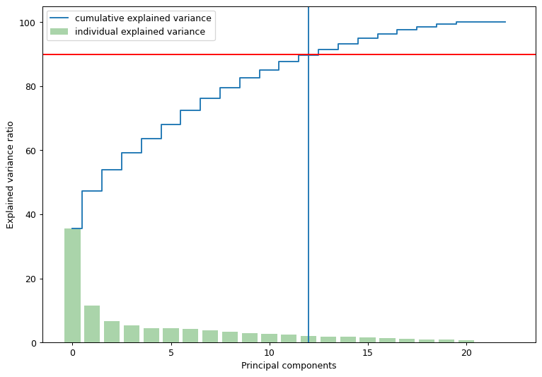
Once the dust has settled and you finally have your cumulative variance, you can assess the dimensional reduction

From the plot above, it can be seen that approximately 90% of the variance can be explained with the 14 principal components. Therefore for the purposes of this notebook, let’s implement PCA with 13 components

Simple visual check, all of your new variables should be linearly independent :


Clustering step

Now that I have reduced the attributes to three dimensions, I will be performing clustering via Agglomerative clustering. Agglomerative clustering is a hierarchical clustering method. It involves merging examples until the desired number of clusters is achieved.

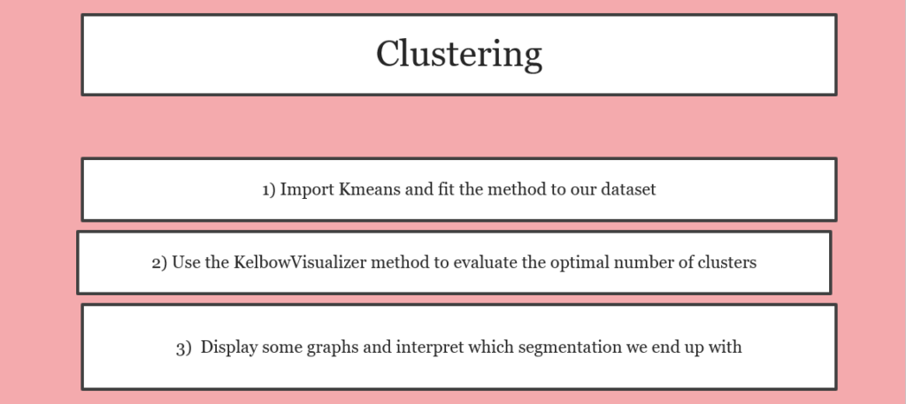
Steps involved in the Clustering

  • Elbow Method to determine the number of clusters to be formed
  • Clustering via Agglomerative Clustering
  • Examining the clusters formed via scatter plot


Use the clustering for profiling :

Now that we have used the clustering method we can use those clusters as a new variable in our original Dataset :

Income vs spending plot shows the clusters pattern :

  • group 0: high spending & average income
  • group 1: high spending & high income
  • group 2: low spending & average income
  • group 3: low spending & low income

Leave a Comment

Your email address will not be published. Required fields are marked *